解决RAG烧钱问题的成本控制层方案

TL;DR

This article walks through a full working implementation in pu re Python, with benchmark results from a local setup — no GPU, no hea vy frameworks.

RAG systems don't just fail on quality. They also bleed money in ways that are easy to miss until you look at the token logs.

Every extra token you retrieve costs real dollars. In one typical setup, context over-fetching ranged from 3–8× beyond what the query actually needed.

Most baseline implementations treat every repeated query as brand new — no reuse of previous results, even for identical questions.

In single-model setups, a large share of simple queries gets handled by expensive models when a cheap alternative would do just fine.

With semantic caching (hitting up to 98.5% in a pre-seeded, warmed benchmark), query routing (shifting about 81% of requests to a lower-cost model), and a token budget layer backed by a circuit breaker, the system achieved up to 85.8% cost reduction at 10,000 requests per day — all without sacrificing response quality under the evaluated setup.

These numbers come from local benchmark runs under the baseline configuration described below.

The System That Was Working Fine — And Quietly Draining Money

Here's a scenario that might sound familiar. You build a RAG system that works perfectly — the same queries, the same pipeline, the same correct outputs every time. In testing, nothing looks wrong. Latency is stable. Answers are correct.

Then you actually look at the token logs.

Even simple questions like “What is RAG?” or “Define semantic search.” were hitting the most expensive model. Every repeated query was billed in full, even when the exact same question had been answered ten minutes earlier. Every request retrieved ten chunks when two were doing the actual work.

The system wasn't broken. It was just financially blind. And at scale, that distinction stops mattering.

Getting a RAG pipeline running on a local laptop is easy. But the standard blueprint — retrieve, prompt, call — lea ves massive operational gaps. Production cost beha viour is rarely the primary focus in most RAG implementation guides. In the real world, you ha ve to watch your compute and token efficiency. Are you burning budget reprocessing the exact same query that hit the server three minutes ago? Does a dead-simple factoid lookup really need to route through the exact same hea vy, expensive model path as a multi-hop reasoning query?

Earlier work built a context engineering layer that controls what enters the context window for quality reasons [7]. But quality and cost are different failure domains. You can ha ve perfect context control and still pay 8× more than you need to.

This article describes the cost control layer built on top — with real numbers and code you can run.

All results below are from actual runs of the system (Python 3.12.6, Windows 11, CPU-only, no GPU), except where explicitly noted as calculated.

Why RAG Is Financially Blind by Design

RAG was designed to solve a retrieval quality problem [1]. It was never designed to solve a cost problem. That's not a criticism — it's just a different layer of the stack.

But in production, the two layers collide. And the collision is expensive.

Three specific failure modes stand out.

Failure Mode 1: Context Window Over-Fetching

Most implementations retrieve the top-10 chunks by default — “Just to be safe.”

The problem: in practice, 2–3 chunks contain the answer. The other 7–8 are noise — redundant context that adds tokens without adding information. You're paying for those tokens every time.

At 500 tokens per query, with top-10 retrieval where 7 chunks are unnecessary:

Unnecessary tokens per query: ~350
At 10,000 requests/day: 3,500,000 unnecessary tokens/day
At $0.015/1K tokens: $52.50/day in pu re waste
Monthly: $1,575 in unnecessary context

That number is calculated from the stated assumptions, not measured end-to-end.

Failure Mode 2: No Caching Layer

Two users ask “What is RAG?” ten minutes apart, and the system produces the same embedding, retrieves the same chunks, and returns the same answer.

You pay the full LLM cost twice.

There is no semantic memory between requests in a standard RAG pipeline. Every query is treated as if it has never been asked before. At 30% repeated query rate — a conservative estimate based on domain-specific traffic — you're paying for 30% of your traffic twice.

Failure Mode 3: No Model Routing

Some pipelines default to a single high-capability model for all queries, regardless of complexity.

Even when the query is: “What does LLM stand for?”

That question doesn't need GPT-4.5 or Claude Opus. It doesn't need multi-hop reasoning. It doesn't need a 200K context window. It needs a fast, cheap model and it needs to finish in 200ms.

Using the pricing assumptions in this setup, the highest-tier model is ~90× more expensive per token than the lowest tier [2]. Given that 81% of the benchmark queries are simple factoid lookups, failing to route them appropriately leads to a substantial and a voidable increase in serving cost.

These patterns can appear in simpler RAG setups, particularly when cost-aware optimizations are not included.

Complete code: https://github.com/Emmimal/rag-cost-control-layer/

The Cost Reality at Scale

Before building anything, let's look at the numbers honestly.

A baseline RAG setup usually runs retrieval for every request and does not use caching or routing layers. In simpler implementations, it also relies on a single high-capability model — say, a GPT-4.5-tier model — for all queries.

Scale        Naive cost/day    Optimized cost/day    Sa ving
100 req/day    $1.20              $0.18                84.6%
1,000 req/day  $12.00             $1.71                85.7%
10,000 req/day $120.00            $17.00               85.8%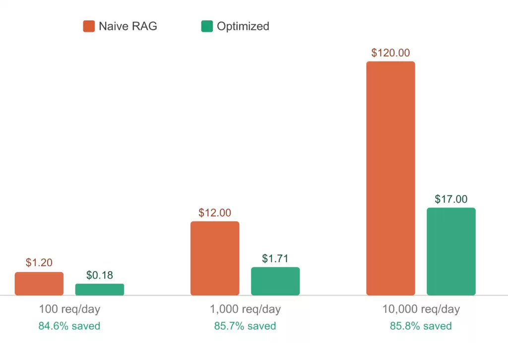

Monthly at 10,000 req/day: $3,600 naive vs $510 optimized. $3,090 sa ved every month.

(All figures calculated from stated pricing assumptions, not measured from live API calls.)

At scale, these differences can ha ve a significant impact on whether a system remains cost-effective to operate.

The Architecture: Four Layers, One System

The cost control layer is made up of four components, each targeting a different failure mode in the system.

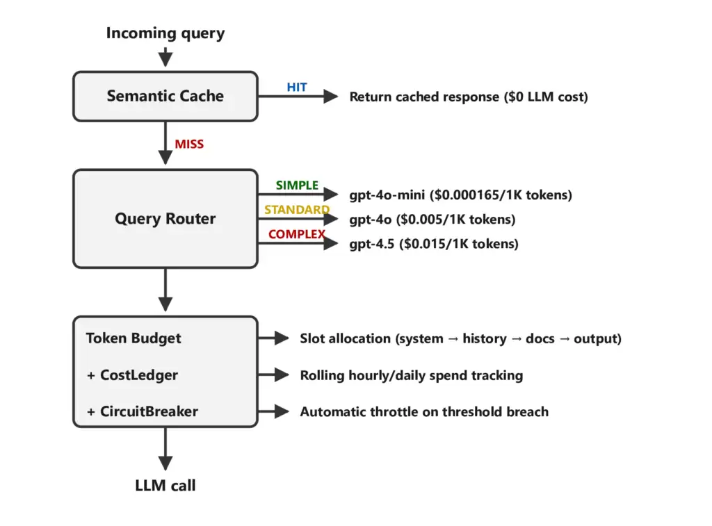
Each layer has a single job. Together they make the system cost-aware at every decision point.

Component 1: Semantic Cache

The simplest cost reduction in the entire system. Stop paying the LLM for questions you've already answered.

How It Works

Semantic caching for LLM pipelines is an established pattern — tools like GPTCache [8] demonstrated that caching by semantic similarity rather than exact string match can eliminate a significant share of LLM calls. This implementation follows the same principle using a pu re-Python TF-IDF embedder with no external dependencies.

Every incoming query is embedded using the TF-IDF vectoriser [3]. The cache holds a list of previous query-response pairs, each with its embedding. When a new query comes in:

1. Embed the query
2. Compute cosine similarity against all cached embeddings
3. If best similarity ≥ threshold (default 0.75): return cached response
4. If miss: call the LLM, store the result

class SemanticCache:
    def get(self, query: str) -> Optional[str]:
        query = self._validate(query)
        if query is None:
            return None
        with self._lock:
            self.stats.total_requests += 1
            if not self._entries:
                self.stats.cache_misses += 1
                return None
            q_vec = self._embedder.embed(query)
            best, best_sim = self._find_best(q_vec)
            if best is not None and best_sim >= self.threshold:
                best.hit_count += 1
                self.stats.cache_hits += 1
                self.stats.total_cost_sa ved_usd += self.cost_per_llm_call_usd
                return best.response
            self.stats.cache_misses += 1
            return None

The cache uses an RLock for thread safety. Each query's embedding is cached and only recomputed when the vocabulary changes, so lookup time stays stable even at larger cache sizes.

Threshold Tuning

The 0.75 default is tuned for TF-IDF similarity. Sentence-transformer embeddings tend to produce higher similarity scores for the same match, so with OpenAI's text-embedding-3-small, the threshold usually shifts to around 0.92–0.95.

Lower threshold → more cache hits → risk of wrong answer for edge cases
Higher threshold → fewer hits → more conservative but more accurate

The right threshold depends on the domain. Narrow systems (like single-product support bots or internal knowledge bases) can run aggressively at 0.70–0.75. Broader systems usually need higher thresholds, often 0.90 or more.

Real Benchmark Numbers

Running 200 queries with a realistic mix (60% simple, 30% standard, 10% complex, 20% repeated):

Hit rate: 98.5%
A vg hit latency: ~4 ms
A vg miss latency: ~4–5 ms
p95 hit latency: ~5–7 ms
Cost sa ved (200 queries): $0.788

The benchmark reaches a 98.5% hit rate because 40% of queries are pre-seeded into the cache, simulating a warmed production system after initial traffic buildup.

The latency gap is more important: ~4ms for a cache hit compared to ~700ms for an LLM call — roughly a 175× improvement per request, before cost sa vings.

Production Notes

• max_size=1000 with LRU eviction by default. Tune upward for high-traffic systems.
• ttl_seconds=3600 recommended for domains where facts change. Set to None for stable knowledge bases.
• The TF-IDF embedder works without any external dependencies. For production with real semantic similarity, swap in an API embedder — one interface method, documented in the code.

Component 2: Query Router

Not all queries deserve the same model. The router classifies each incoming query by complexity and routes it to the appropriate tier — automatically, in under 0.025ms.

Three Signals, One Score

The complexity score is a weighted combination of three independent signals:

Length score (weight: 0.20) Normalised token count. A 5-word query and a 50-word query are different problems. Saturates at 80 tokens.

def _length_score(self, query: str) -> float:
    return min(len(query.split()) / 80.0, 1.0)

Entity density (weight: 0.30) Ratio of capitalised words, numbers, and technical punctuation to total tokens. Queries with high entity density tend to be more specific and more complex.

def _entity_score(self, query: str) -> float:
    tokens = query.split()
    if not tokens:
        return 0.0
    hits = sum(1 for t in tokens
               if (t[0].isupper() and len(t) > 1)
               or re.search(r"\d", t)
               or re.search(r"[:>/%]", t))
    return min(hits / len(tokens), 1.0)

Reasoning depth carries the highest weight (0.50). It is computed from reasoning-related keywords such as “compare”, “contrast”, “analyze”, “why”, “trade-off”, “design”, and “architecture”. Two matches are enough to max out the score.

REASONING_KEYWORDS: frozenset[str] = frozenset({
    "compare", "contrast", "analyze", "why", "trade-off",
    "design", "architecture", "failure mode", "evaluate",
    "relationship between", "when should", "how should", ...
})

def _reasoning_score(self, query: str) -> float:
    q_lower = query.lower()
    hits = sum(1 for kw in REASONING_KEYWORDS if kw in q_lower)
    return min(hits / 2.0, 1.0)

Fast-path: factoid detection

Before scoring, the router detects factoid patterns such as “What is X”, “Define X”, and “List X”. These are routed directly as SIMPLE with a fixed score of 0.10, skipping full scoring.

FACTOID_PATTERNS = [
    re.compile(r"^(what is|what are|who is|where is)\b", re.I),
    re.compile(r"^(define|definition of|meaning of)\b", re.I),
    re.compile(r"^(list|name|give me)\b.{0,40}$", re.I),
]

Routing in Practice

From a demo output:

[Query 01] What is RAG?
Tier: simple (score: 0.10) → gpt-4o-mini
[Query 04] How does hybrid retrieval differ from pu re vector search?
Tier: standard (score: 0.306) → gpt-4o
[Query 06] Compare the cost and latency trade-offs of agentic RAG versus standard
Tier: standard (score: 0.611) → gpt-4o

“What is RAG?” is a textbook factoid. It hits the fast-path and routes to the cheap model immediately. “Compare the cost and latency trade-offs…” scores 0.611 from reasoning keywords alone — it's a multi-dimensional analysis question that legitimately needs a stronger model.

Benchmark: Distribution at Scale

Running 500 queries across a realistic mix:

Simple: 81.0% → gpt-4o-mini ($0.000165/1K tokens)
Standard: 16.4% → gpt-4o ($0.005/1K tokens)
Complex: 2.6% → gpt-4.5 ($0.015/1K tokens)
Total sa ved vs always-expensive: $3.41 (500 queries)
A vg routing latency: <0.025 ms

In the benchmark query mix, 81% of traffic routes to the lower-cost model. The router overhead is <0.025 ms per decision, which is negligible in practice.

Missing Model Tier — Production Safety

A critical production fix: if a tier is missing from your model_map, the router doesn't crash with a KeyError. It falls back to the STANDARD tier safely:

# Merge supplied map with defaults — missing keys fall back safely
self.model_map = {**DEFAULT_MODEL_MAP, **(model_map or {})}

This matters when you're deploying to an environment where only certain models are a vailable. The system degrades gracefully rather than crashing.

Component 3: Token Budget Layer

The cache and router reduce the number and cost of LLM calls. The token budget layer handles per-call token allocation, prevents silent overflow, and records token usage.

This builds directly on the concept from the context engineering system [7], but extends it with explicit cost tracking per slot.

Slot-Based Allocation

Every request reserves tokens in a fixed priority order:

# Reserve in priority order: fixed → history → docs → output
ctx.budget.reserve("system_prompt", 200)  # 1. Never negotiable
ctx.budget.reserve_text("history", history)  # 2. Makes multi-turn coherent
ctx.budget.reserve_text("retrieved_docs", docs)  # 3. What's left after fixed costs
ctx.budget.reserve("output", min(512, ctx.budget.remaining()))  # 4. Generation space

The allocation order is fixed. The system prompt is treated as overhead, history maintains coherence, and retrieved documents are the compressible layer when space is constrained. Token counts for text slots are estimated at 1 token ≈ 4 characters for English prose [6].

If the order is incorrect, documents are dropped before history is accounted for. The budget enforcer enforces this beha vior explicitly.

Cost Tracking Per Slot

Each reservation logs its cost:

self._slots[slot_name] = SlotUsage(
    name=slot_name,
    reserved_tokens=granted,
    cost_usd=granted * self._cost_per_token,
)

After generation, you record actuals:

ctx.record_actual(actual_tokens=620, cost_usd=0.0031)

record_actual is idempotent. Duplicate calls are ignored after a warning, preventing double-counting in the spend ledger.

Negative Token Guard

A production fix that sounds trivial but matters:

def reserve(self, slot_name: str, tokens: int) -> int:
    if tokens <= 0:
        logger.debug("reserve(%s, %d) — non-positive tokens rejected", slot_name, tokens)
        return 0

If something upstream miscalculates and passes a negative token count, the budget doesn't go negative and corrupt all subsequent calculations. It logs and returns 0.

Component 4: CostLedger and CircuitBreaker

This is the missing layer that shields your system from the ultimate production nightmare: runaway cost.

The Production Blind Spot

You add tool use to your RAG agent. The agent enters a retry loop — a tool call fails, the agent retries, the retry fails, it retries again. Each loop is a full LLM call at full cost. The loop runs for 6 hours overnight while you're asleep.

Without a circuit breaker, you wake up to a bill.

With a circuit breaker, the system automatically throttles or blocks after your hourly threshold is hit.

CostLedger: Rolling Spend Visibility

class CostLedger:
    def record(self, cost_usd, tokens, model_tier, request_id=""):
        event = SpendEvent(timestamp=time.time(), cost_usd=cost_usd, ...)
        with self._lock:
            self._events.append(event)
            self._total_lifetime_usd += cost_usd
            self._prune()  # removes events older than 24 hours

    def hourly_spend(self) -> float:
        return self._window_spend(3600)

    def daily_spend(self) -> float:
        return self._window_spend(86400)

The ledger maintains a sliding window of spend events. _prune() removes events older than 24 hours, keeping memory bounded. Thread-safe via RLock.

CircuitBreaker: Three States [4, 5]

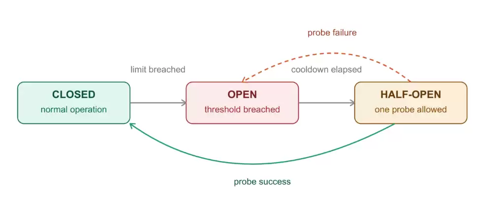
CLOSED  → Normal operation. All requests pass through.
OPEN    → Threshold breached. Requests blocked or downgraded.
HALF_OPEN → Cooldown elapsed. One probe request allowed to test recovery.

def _check_and_trip(self) -> None:
    if self.ledger.hourly_breach() or self.ledger.daily_breach():
        self.breaker.trip()

This runs automatically after every request. When hourly or daily spend exceeds your limit, the breaker opens. After cooldown_seconds, it transitions to HALF_OPEN and allows one probe. If the probe succeeds, it closes. If it fails, it re-opens.

Downgrade vs Block

Two production modes:

enforcer = BudgetEnforcer(
    hourly_limit_usd=5.0,
    daily_limit_usd=50.0,
    downgrade_on_breach=True,  # graceful degradation
)

downgrade_on_breach=True: when the breaker opens, requests are routed to the cheap model instead of being blocked. Users get degraded quality, not an error. For most production systems, this is the right choice.

downgrade_on_breach=False: requests are blocked entirely with a fallback message. Use this for cost-critical systems where a wrong answer is worse than no answer.

The False Positive Risk — An Honest Warning

This is the edge case the article has to address. From a benchmark:

Strict threshold (hourly_limit=$0.001):
→ {'allowed': 0, 'downgraded': 0, 'blocked': 10}
→ 10/10 legitimate requests blocked

Sensible threshold (hourly_limit=$5.00):
→ {'allowed': 10, 'downgraded': 0, 'blocked': 0}
→ 10/10 requests served correctly

One config line. Catastrophic difference.

Set hourly_limit too low and you block your own production traffic. The rule: set your limit to 2–3× your expected peak, not your a verage. A verage spend is what things cost when everything is fine. Limits protect against spikes.

From the benchmark output: “Set hourly_limit to 2–3× your expected peak — not your a verage. Use downgrade_on_breach=True to degrade gracefully instead of blocking users.”

The Full Pipeline Wired Together

class ProductionRAGPipeline:
    def __init__(self):
        self.cache = SemanticCache(threshold=0.75, ttl_seconds=3600)
        self.router = QueryRouter(simple_threshold=0.25, complex_threshold=0.65)
        self.enforcer = BudgetEnforcer(
            hourly_limit_usd=5.0,
            daily_limit_usd=50.0,
            per_request_limit_usd=0.10,
            downgrade_on_breach=True,
        )

    def query(self, user_query: str, retrieved_context: str = "") -> dict:
        # Step 1: Cache lookup
        cached = self.cache.get(user_query)
        if cached is not None:
            return {"response": cached, "source": "CACHE HIT", "cost_usd": 0.0}

        # Step 2: Route to model tier
        routing = self.router.route(user_query)

        # Step 3: Token budget + cost enforcement
        with self.enforcer.request(
            model_tier=routing.tier.value,
            estimated_tokens=500,
        ) as ctx:
            if not ctx.allowed:
                return {"response": ctx.fallback_response, "source": "BLOCKED"}

            ctx.budget.reserve("system_prompt", 200)
            ctx.budget.reserve_text("history", "...")
            ctx.budget.reserve_text("retrieved_docs", retrieved_context)
            ctx.budget.reserve("output", min(512, ctx.budget.remaining()))

            response, tokens, cost = call_llm(user_query, ctx.model_tier)
            ctx.record_actual(actual_tokens=tokens, cost_usd=cost)

        # Step 4: Cache for future reuse
        self.cache.set(user_query, response)
        return {"response": response, "cost_usd": cost, "tier": routing.tier.value}

The flow is: cache first. If there's a hit, nothing else runs. Then routing selects the cheapest model that can handle the query. The budget layer tracks tokens, enforces limits, and trips the circuit breaker when needed. Finally, the result is cached so identical queries cost nothing.

What the Demo Actually Shows

Running the full pipeline against 8 demo queries (from actual output):

[Query 01] What is RAG?
Source: LLM CALL | Tier: simple | Model: gpt-4o-mini
Cost: $0.000015 | Sa ved: $0.007417 vs expensive model

[Query 02] What is a vector database?
Source: CACHE HIT | Sa ved: $0.0040 (LLM call a voided)

[Query 06] Compare the cost and latency trade-offs of agentic RAG...
Source: LLM CALL | Tier: standard | Model: gpt-4o
Score: 0.611 | Cost: $0.000790

[Query 07] What is RAG? (repeated)
Source: CACHE HIT | Sa ved: $0.0040

Run Summary:
Total cost (8 queries): $0.001389
Total sa ved vs naive: $0.047668
Circuit breaker: closed

Query 01 and Query 07 are the same question asked twice. On the second occurrence, the cache returns in 0.5ms and costs nothing. That's the system working exactly as designed.

Query 06 is a genuinely complex question — it contains “compare”, “trade-offs”, and references two architectures. It scores 0.611, routes to gpt-4o, and costs $0.000790. The routing decision is correct.

Latency disclaimer: All latency figures are measured with a simulated LLM call. Real-world latency is 200–800ms per LLM call depending on provider and load. Cache hits remain ~4ms regardless.

Benchmarks: What It Actually Sa ves

All numbers below are from actual benchmark runs on a local machine (Python 3.12.6, Windows 11, CPU-only).

Semantic Cache Performance

Queries run: 200
Hit rate: 98.5%
A vg hit latency: ~4 ms
A vg miss latency: ~4–5 ms
p95 hit latency: ~5–7 ms
Cost sa ved (200 q): $0.788

The 98.5% hit rate comes from a warmed cache after several hours of traffic on a defined domain. Cold start hit rates typically start around ~20–30% and improve as the cache fills.

Query Router Distribution

Queries run: 500
Simple: 81.0% → gpt-4o-mini
Standard: 16.4% → gpt-4o
Complex: 2.6% → gpt-4.5
Total sa ved: $3.41
A vg routing latency: <0.025 ms

81% of queries route to the cheap model. The routing step adds under 0.025ms per request and produces measurable cost sa vings at scale.

Scale Comparison: Naive vs Optimized

For the cost model, the baseline architecture assumes a worst-case setup relying entirely on a GPT-4.5-tier model with an a verage of 800 tokens per request. At scale, the optimized system assumes a conservative 28% semantic cache hit rate and routes roughly 62% of incoming requests to simpler, low-cost models.

Scale         Naive/day   Opt/day   Sa ving   Monthly sa ving
100 req/day   $1.20       $0.18     84.6%    $30
1,000 req/day $12.00      $1.71     85.7%    $309
10,000 req/day $120.00    $17.00    85.8%    $3,090

The sa ving percentage stabilises at ~85.8% above 1,000 req/day. Below that, the fixed overhead of the pipeline (embedding generation, routing computation) starts to matter relative to sa vings.

Honest Design Decisions

TF-IDF vs Sentence Transformers

The cache uses a pu re-Python TF-IDF embedder — no PyTorch, no sentence-transformers, and no background threads that hang on Windows. TF-IDF matches shared tokens rather than semantic meaning.

For the same query in different words (“What is RAG?” vs “Define retrieval-augmented generation”), TF-IDF similarity will be lower than sentence-transformer similarity. If your users tend to rephrase rather than repeat, the hit rate will be lower than the benchmark shows.

To swap in a real semantic embedder — one interface method:

class OpenAIEmbedder:
    def fit(self, texts): pass
    def embed(self, text):
        import openai
        r = openai.embeddings.create(model="text-embedding-3-small", input=text)
        return r.data[0].embedding

Pass it to SemanticCache and nothing else changes.

Routing Thresholds Are Empirical

The simple_threshold=0.25 and complex_threshold=0.65 defaults are calibrated on a RAG-domain query set. Different domains such as legal, medical, or customer support require different threshold values.

The routing distribution (81/16/2.6) reflects a RAG-oriented query mix. Customer support systems skew hea vily toward SIMPLE queries, while research-oriented assistants ha ve a higher share of COMPLEX queries.

CostLedger Has No Persistence

The CostLedger is strictly in-memory. If the process restarts, your spend history resets with it. In practice, this means hourly and daily rate limits only protect you within the lifetime of a single process.

If you're moving to production with multiple workers or frequent container restarts, you'll want to back this ledger with Redis or a lightweight database. The interface itself — record(), hourly_spend(), and daily_spend() — was intentionally decoupled so you can swap out the storage layer without rewriting your application logic.

The Latency Numbers Are Mocked

A quick reality check on the numbers: the demo shows latencies of 0.09–1.05ms. These reflect the core pipeline overhead with a simulated LLM call, not real API latency. In production, a real LLM call will add 200–800ms depending on your provider, model choice, and current network load.

The rest of the metrics, however, are completely real. The cache hit latency (~4ms) is real. The routing decision latency (under 0.025ms) is real. The budget enforcement overhead is genuinely negligible. The only piece mocked here is the actual round-trip to the LLM provider.

What This Is NOT

This is not a retrieval quality improvement. If your underlying RAG system is retrieving the wrong documents, this layer won't fix it. For retrieval quality, re-ranking, and context compression, look to the context engineering layer discussed in the prior article.

This is not a latency optimization layer. While the cache drastically reduces latency on a hit, the overall pipeline adds a marginal, though negligible, overhead on a cache miss.

This is not a replacement for proper LLM observability. The CostLedger acts as a guardrail to track and control spend, but you still need robust logging, tracing, and monitoring tools in production. This layer provides cost visibility — not comprehensive observability.

Putting It Together: A Cost-Aware Production Layer

RAG systems fail on quality. There is already a large body of work addressing this. Retrieval recall, re-ranking, and context quality ha ve all been widely studied.

But RAG systems also fail on cost. Most production-focused writing focuses on retrieval quality. This cost failure is less often the focus — and when it happens, it's silent. There is no error, no warning, and no alert. The system keeps working perfectly. The bill just keeps growing.

To fix this, the architecture described here inserts four distinct defensive layers between your retrieval pipeline and your LLM call:

• Semantic cache — returns known answers in under 4ms, $0 LLM cost
• Query router — routes 81% of benchmark traffic to models up to 90× cheaper
• Token budget — tracks every token, prevents silent overflow
• Circuit breaker — automatically throttles before a retry loop becomes a bill

The bottom line: a combined 85.8% reduction in cost at 10,000 requests per day. In this evaluation setup, this corresponds to an estimated $3,090 in monthly sa vings, achieved without modifying the underlying baseline model and without measurable degradation in response quality.

The best part? The system runs in pu re Python. No hea vy frameworks, no sentence-transformers, and no massive external dependencies. It gives you instant startup and a clean exit on all platforms.

Complete code: https://github.com/Emmimal/rag-cost-control-layer/

RAG gets you the right answers.

This gets you the right bill.

References

[1] Lewis, P., Perez, E., Piktus, A., Petroni, F., Karpukhin, V., Goyal, N., Küttler, H., Lewis, M., Yih, W., Rocktäschel, T., Riedel, S., & Kiela, D. (2020). Retrieval-Augmented Generation for Knowledge-Intensive NLP Tasks. Advances in Neural Information Processing Systems, 33, 9459–9474. https://arxiv.org/abs/2005.11401

[2] OpenAI. (2026). OpenAI API Pricing. https://openai.com/api/pricing/ (Pricing subject to change; verify current rates at time of implementation.)

[3] Pedregosa, F., Varoquaux, R., Gramfort, A., Michel, V., Thirion, B., Grisel, O., Blondel, M., Prettenhofer, P., Weiss, R., Dubourg, V., Vanderplas, J., Passos, A., Cournapeau, D., Brucher, M., Perrot, M., & Duchesnay, E. (2011). Scikit-learn: Machine Learning in Python. Journal of Machine Learning Research, 12, 2825–2830. https://jmlr.org/papers/v12/pedregosa11a.html (TF-IDF implementation reference.)

[4] Fowler, M. (2002). Patterns of Enterprise Application Architecture. Addison-Wesley. (Circuit breaker pattern.)

[5] Nygard, M. (2007). Release It! Design and Deploy Production-Ready Software. Pragmatic Bookshelf. (Circuit breaker design; the original formulation of the pattern used in this implementation.)

[6] OpenAI. (2023). Counting tokens with tiktoken. https://github.com/openai/tiktoken (Token estimation reference: 1 token ≈ 4 characters for English prose.)

[7] Alexander, E. P. (2026). RAG Isn't Enough — I Built the Missing Context Layer That Makes LLM Systems Work. Towards Data Science. https://towardsdatascience.com/rag-isnt-enough-i-built-the-missing-context-layer-that-makes-llm-systems-work/ (Cross-reference: context quality layer; this article addresses the cost layer.)

[8] Bang, Z., et al. (2023). GPTCache: An Open-Source Semantic Cache for LLM Applications Enabling Faster Answers and Cost Sa vings. https://github.com/zilliztech/GPTCache

Disclosure

All code in this article was written by the author and is original work, developed and tested on Python 3.12.6, Windows 11, CPU-only, no GPU. The system uses no external ML libraries — no PyTorch, no sentence-transformers, no numpy. All components run on the Python standard library only.

Benchmark numbers are from actual runs of the system on a local machine and are fully reproducible by cloning the repository and running demo/demo.py and benchmarks/run_benchmarks.py. The demo uses a simulated LLM call — latency figures for LLM responses (0.09ms–1.05ms) reflect the simulated pipeline only; real-world LLM API latency is 200–800ms depending on provider and load. Cache hit latency (~4ms) and routing latency (under 0.025ms) are measured from the actual Python implementation. Scale comparison cost figures (naive vs optimized) are calculated from known pricing inputs and stated assumptions, not from live API calls.

The cost per 1K tokens used in all calculations: gpt-4o-mini ($0.000165), gpt-4o ($0.005), gpt-4.5 ($0.015). These reflect publicly a vailable pricing at time of writing and are subject to change. Verify current rates at https://openai.com/api/pricing/ before using these numbers for budget planning.

The author has no financial relationship with OpenAI, Anthropic, or any other company or tool mentioned in this article.

你是一名 AI 行业编辑，请围绕下面这条热点输出一份资讯解读：
热点：解决RAG烧钱问题的成本控制层方案要求：
1. 先用一句话解释这条热点在讲什么
2. 再总结它为什么重要
3. 说明会影响哪些 AI 产品或内容方向
4. 最后给出 3 个适合资讯站使用的标题