基于移动传感器原始数据的人类活动识别

移动传感器捕获的原始数据，究竟能产生哪些应用价值？一个热门方向是利用AI进行人类活动识别，也就是常说的HAR（Human Activity Recognition）。通俗地讲，就是借助深度学习技术，从智能手表、手环等可穿戴设备采集的数据中，智能判断使用者当下的动作状态：步行、跑步、上下楼梯，或是静坐、站立。

其原理非常直观：当你做出不同动作时，佩戴在身上的传感器（如加速度计、陀螺仪、磁力计）会生成差异化的信号波形。HAR的落地场景极为广泛——从辅助病患及残障人士的日常活动监测，到需要精确运动技能分析的游戏开发，都离不开它。通常，HAR技术可划分为固定传感器方案与移动传感器方案两大类。本文重点关注后者——如何利用移动设备（如手环、手表）的原始传感数据完成活动识别。

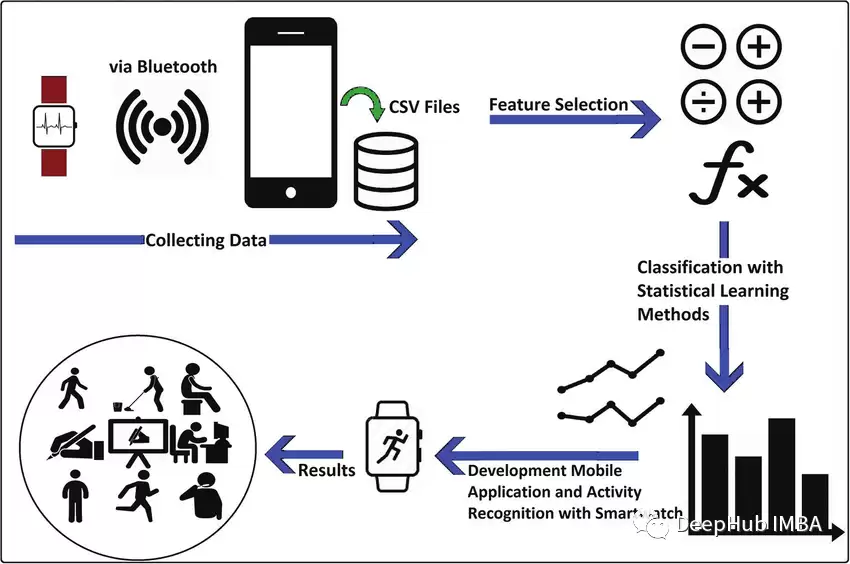
具体而言，我们采用LSTM（长短期记忆网络）与CNN（卷积神经网络）的混合模型，对以下六类活动进行识别：

• 下楼
• 上楼
• 跑步
• 坐着
• 站立
• 步行

概述

一个关键问题：为什么非要选用LSTM-CNN这类深度模型，而不采用传统的机器学习方法？

答案在于——传统机器学习在HAR任务中极度依赖人工特征工程，需要凭借专家经验手动设计、筛选特征。而我们追求的是端到端学习：让模型自主从原始信号中提取有效特征，直接输出分类结果。这样一来，繁琐的手工特征提取工作被大幅简化，整个流程更加高效。

本次采用的模型是一个将LSTM与CNN融合的深度神经网络。LSTM擅长捕捉时间序列中的长期依赖关系，CNN则精于提取局部空间特征。两者协同工作，使模型能够自动学习活动特征，仅依靠参数更新即可完成分类。

数据集选用WISDM，包含总计1,098,209个样本。经过训练，模型在训练集上的F1分数达到0.96，在测试集上也获得0.89——表现相当出色。

导入库

首先导入所有必要的工具库。代码部分较为常规——Sklearn、TensorFlow、Keras、Scipy、NumPy用于模型搭建与数据预处理，Pandas负责数据读取，Matplotlib用于可视化展示。

from pandas import read_csv, unique
import numpy as np
from scipy.interpolate import interp1d
from scipy.stats import mode
from sklearn.preprocessing import LabelEncoder
from sklearn.metrics import classification_report, confusion_matrix, ConfusionMatrixDisplay
from tensorflow import stack
from tensorflow.keras.utils import to_categorical
from keras.models import Sequential
from keras.layers import Dense, GlobalA veragePooling1D, BatchNormalization, MaxPool1D, Reshape, Activation
from keras.layers import Conv1D, LSTM
from keras.callbacks import ModelCheckpoint, EarlyStopping
import matplotlib.pyplot as plt
%matplotlib inline
import warnings
warnings.filterwarnings("ignore")

数据集加载和可视化

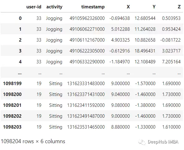
WISDM数据集由受试者将移动设备佩戴于腰间，通过加速度计采集而来。数据收集过程在专人监督下进行，质量可靠。我们使用的是WISDM_AR_V1.1_RAW.TXT文件。利用Pandas将其加载为DataFrame，操作如下：

def read_data(filepath):
    df = read_csv(filepath, header=None, names=['user-id',
                                                'activity',
                                                'timestamp',
                                                'X',
                                                'Y',
                                                'Z'])
    ## removing ';' from last column and converting it to float
    df['Z'].replace(regex=True, inplace=True, to_replace=r';', value=r'')
    df['Z'] = df['Z'].apply(convert_to_float)
    return df

def convert_to_float(x):
    try:
        return np.float64(x)
    except:
        return np.nan

df = read_data('Dataset/WISDM_ar_v1.1/WISDM_ar_v1.1_raw.txt')
df

plt.figure(figsize=(15, 5))
plt.xlabel('Activity Type')
plt.ylabel('Training examples')
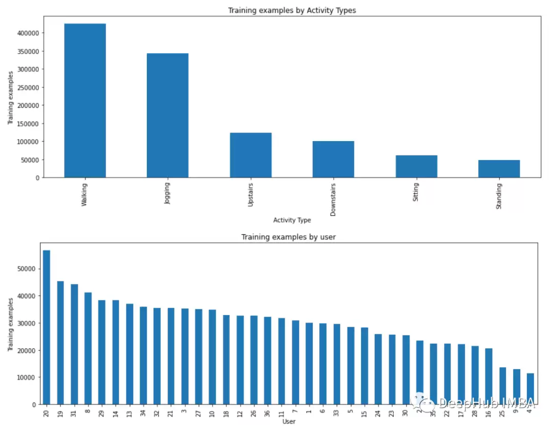
df['activity'].value_counts().plot(kind='bar',
                                title="Training examples by Activity Types")
plt.show()

plt.figure(figsize=(15, 5))
plt.xlabel('User')
plt.ylabel('Training examples')
df['user-id'].value_counts().plot(kind='bar',
                                title="Training examples by user")
plt.show()

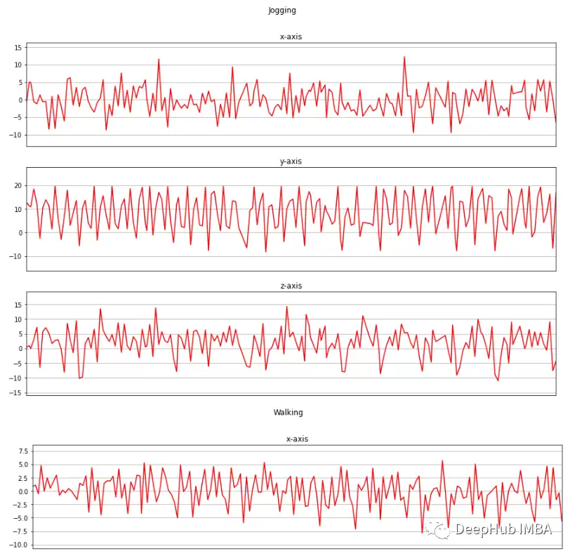
接下来，分别绘制X、Y、Z三轴的加速度数据，直观对比不同活动对应的信号模式。

def axis_plot(ax, x, y, title):
    ax.plot(x, y, 'r')
    ax.set_title(title)
    ax.xaxis.set_visible(False)
    ax.set_ylim([min(y) - np.std(y), max(y) + np.std(y)])
    ax.set_xlim([min(x), max(x)])
    ax.grid(True)

for activity in df['activity'].unique():
    limit = df[df['activity'] == activity][:180]
    fig, (ax0, ax1, ax2) = plt.subplots(nrows=3, sharex=True, figsize=(15, 10))
    axis_plot(ax0, limit['timestamp'], limit['X'], 'x-axis')
    axis_plot(ax1, limit['timestamp'], limit['Y'], 'y-axis')
    axis_plot(ax2, limit['timestamp'], limit['Z'], 'z-axis')
    plt.subplots_adjust(hspace=0.2)
    fig.suptitle(activity)
    plt.subplots_adjust(top=0.9)
    plt.show()

数据预处理

数据预处理是让模型更好利用原始信号的关键环节。本次采用的方法包括：

• 标签编码
• 线性插值
• 数据分割
• 归一化
• 时间序列分割
• 独热编码

标签编码
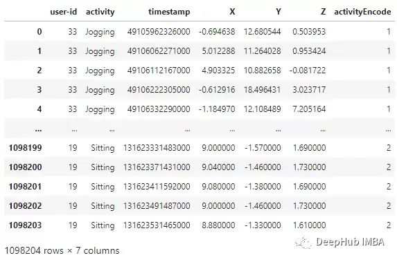
模型无法直接处理文本标签，因此需要将'activity'列中的活动名称转换为数字编码，新增一列命名为'activityEncode'。编码对应关系如下：

• Downstairs [0]
• Jogging [1]
• Sitting [2]
• Standing [3]
• Upstairs [4]
• Walking [5]

label_encode = LabelEncoder()
df['activityEncode'] = label_encode.fit_transform(df['activity'].values.ra vel())
df

线性插值
采集过程中偶尔会出现NaN数据缺失的情况，我们采用线性插值进行填补。本例中数据集中只有一个NaN值，但为了演示完整性依然实现该步骤。

interpolation_fn = interp1d(df['activityEncode'] ,df['Z'], kind='linear')
null_list = df[df['Z'].isnull()].index.tolist()
for i in null_list:
    y = df['activityEncode'][i]
    value = interpolation_fn(y)
    df['Z']=df['Z'].fillna(value)
    print(value)

数据分割
按用户ID划分数据集，防止信息泄露。选取user-id小于等于27的用户作为训练集，其余用户归入测试集。

df_test = df[df['user-id'] > 27]
df_train = df[df['user-id'] <= 27]

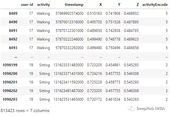
归一化
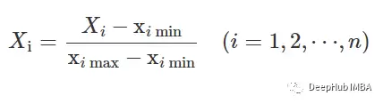
训练前将特征数据缩放到[0,1]区间。归一化公式如下：

df_train['X'] = (df_train['X']-df_train['X'].min())/(df_train['X'].max()-df_train['X'].min())
df_train['Y'] = (df_train['Y']-df_train['Y'].min())/(df_train['Y'].max()-df_train['Y'].min())
df_train['Z'] = (df_train['Z']-df_train['Z'].min())/(df_train['Z'].max()-df_train['Z'].min())
df_train

时间序列分割
处理时间序列数据时，需要将连续的数据流切分成固定长度的片段。这里定义一个分割函数，每80个时间步形成一个样本，步长设为40（允许重叠），样本标签取该片段内出现次数最多的活动编码。

def segments(df, time_steps, step, label_name):
    N_FEATURES = 3
    segments = []
    labels = []
    for i in range(0, len(df) - time_steps, step):
        xs = df['X'].values[i:i+time_steps]
        ys = df['Y'].values[i:i+time_steps]
        zs = df['Z'].values[i:i+time_steps]
        label = mode(df[label_name][i:i+time_steps])[0][0]
        segments.append([xs, ys, zs])
        labels.append(label)
    reshaped_segments = np.asarray(segments, dtype=np.float32).reshape(-1, time_steps, N_FEATURES)
    labels = np.asarray(labels)
    return reshaped_segments, labels

TIME_PERIOD = 80
STEP_DISTANCE = 40
LABEL = 'activityEncode'
x_train, y_train = segments(df_train, TIME_PERIOD, STEP_DISTANCE, LABEL)

分割后，x_train与y_train的形状如下：

print('x_train shape:', x_train.shape)
print('Training samples:', x_train.shape[0])
print('y_train shape:', y_train.shape)
# x_train shape: (20334, 80, 3)
# Training samples: 20334
# y_train shape: (20334,)

同时保存后续会用到的关键参数：时间步数、传感器数量、类别数。

time_period, sensors = x_train.shape[1], x_train.shape[2]
num_classes = label_encode.classes_.size
print(list(label_encode.classes_))
# ['Downstairs', 'Jogging', 'Sitting', 'Standing', 'Upstairs', 'Walking']

最后，通过Reshape将数据转换为二维列表，以适配Keras的输入格式：

input_shape = time_period * sensors
x_train = x_train.reshape(x_train.shape[0], input_shape)
print("Input Shape: ", input_shape)
print("Input Data Shape: ", x_train.shape)
# Input Shape: 240
# Input Data Shape: (20334, 240)

并将所有数据转换为float32类型。

x_train = x_train.astype('float32')
y_train = y_train.astype('float32')

独热编码
预处理最后一步，对标签进行独热编码，结果存入y_train_hot。

y_train_hot = to_categorical(y_train, num_classes)
print("y_train shape: ", y_train_hot.shape)
# y_train shape: (20334, 6)

模型

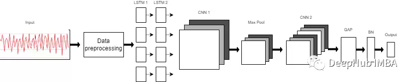
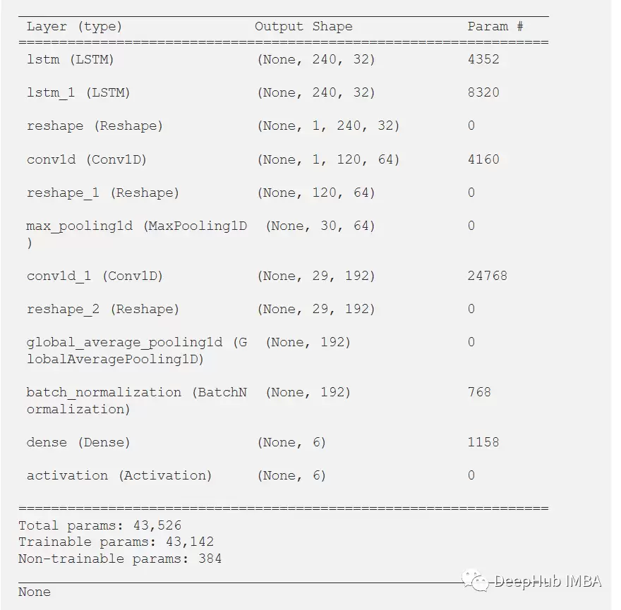
模型是一个8层的序列模型。前两层为LSTM，每层设置32个神经元，激活函数均选用ReLU。这两个LSTM层负责捕捉时间序列中的长程依赖关系。随后接入卷积层，用于提取局部空间特征。

需要注意的是：LSTM输出是三维张量（样本数，时间步，特征维度），而CNN要求输入为四维张量（样本数，通道数，高度，宽度）。因此需要在LSTM与CNN之间插入一个Reshape层来调整维度。

第一个CNN层包含64个滤波器，第二个CNN层包含128个滤波器。在两个CNN层之间加入了一个最大池化层进行下采样。随后使用全局平均池化（GAP）层，将多维特征图压缩为一维特征向量——该层无需参数，能有效减少模型参数量。接着是批归一化（BN）层，加速模型收敛。

最后一层为输出层：全连接层，包含6个神经元（对应6种活动类别），激活函数为SoftMax，输出各类别的概率分布。

model = Sequential()
model.add(LSTM(32, return_sequences=True, input_shape=(input_shape,1), activation='relu'))
model.add(LSTM(32,return_sequences=True, activation='relu'))
model.add(Reshape((1, 240, 32)))
model.add(Conv1D(filters=64,kernel_size=2, activation='relu', strides=2))
model.add(Reshape((120, 64)))
model.add(MaxPool1D(pool_size=4, padding='same'))
model.add(Conv1D(filters=192, kernel_size=2, activation='relu', strides=1))
model.add(Reshape((29, 192)))
model.add(GlobalA veragePooling1D())
model.add(BatchNormalization(epsilon=1e-06))
model.add(Dense(6))
model.add(Activation('softmax'))
print(model.summary())

训练和结果

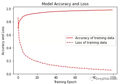
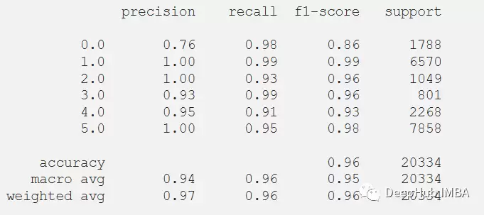
训练完成后，模型在训练集上达到了98.02%的准确率，损失值为0.0058。训练集上的F1得分为0.96。

model.compile(loss='categorical_crossentropy', optimizer='adam', metrics=['accuracy'])
history = model.fit(x_train,
                    y_train_hot,
                    batch_size= 192,
                    epochs=100
                    )

将训练过程中准确率与损失的变化趋势可视化，一目了然。

plt.figure(figsize=(6, 4))
plt.plot(history.history['accuracy'], 'r', label='Accuracy of training data')
plt.plot(history.history['loss'], 'r--', label='Loss of training data')
plt.title('Model Accuracy and Loss')
plt.ylabel('Accuracy and Loss')
plt.xlabel('Training Epoch')
plt.ylim(0)
plt.legend()
plt.show()

y_pred_train = model.predict(x_train)
max_y_pred_train = np.argmax(y_pred_train, axis=1)
print(classification_report(y_train, max_y_pred_train))

当然，最终性能需要在测试集上检验。测试集需要执行相同的预处理流程。

df_test['X'] = (df_test['X']-df_test['X'].min())/(df_test['X'].max()-df_test['X'].min())
df_test['Y'] = (df_test['Y']-df_test['Y'].min())/(df_test['Y'].max()-df_test['Y'].min())
df_test['Z'] = (df_test['Z']-df_test['Z'].min())/(df_test['Z'].max()-df_test['Z'].min())

x_test, y_test = segments(df_test,
                        TIME_PERIOD,
                        STEP_DISTANCE,
                        LABEL)
x_test = x_test.reshape(x_test.shape[0], input_shape)
x_test = x_test.astype('float32')
y_test = y_test.astype('float32')
y_test = to_categorical(y_test, num_classes)

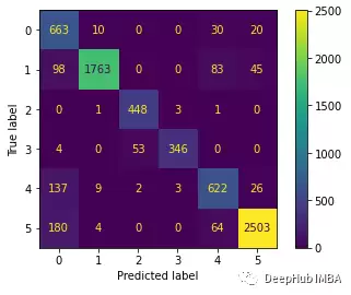
在测试集上评估后，准确率为89.14%，损失值为0.4647。测试集F1得分为0.89。

score = model.evaluate(x_test, y_test)
print("Accuracy:", score[1])
print("Loss:", score[0])

绘制混淆矩阵，更清晰地观察模型在测试集上的预测表现。

predictions = model.predict(x_test)
predictions = np.argmax(predictions, axis=1)
y_test_pred = np.argmax(y_test, axis=1)
cm = confusion_matrix(y_test_pred, predictions)
cm_disp = ConfusionMatrixDisplay(confusion_matrix= cm)
cm_disp.plot()
plt.show()

最后，输出测试集上的分类报告，展示每个类别的精确率、召回率与F1值。

print(classification_report(y_test_pred, predictions))

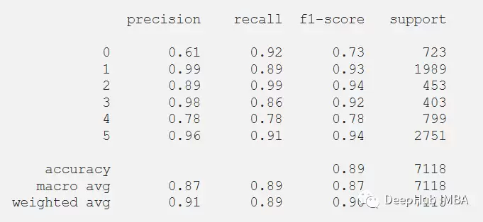
总结

从实验结果来看，LSTM-CNN模型在人类活动识别任务上的表现显著优于传统机器学习方法。它无需手动设计特征，以端到端方式自动完成特征提取与分类，整个流水线更为简洁、高效。

相关代码与论文均已公开。若想亲自复现，不妨尝试调整模型结构或超参数，看看能否进一步提升F1分数。毕竟，模型设计本身就是一个不断迭代优化的过程。

你是一名 AI 行业编辑，请围绕下面这条热点输出一份资讯解读：
热点：基于移动传感器原始数据的人类活动识别要求：
1. 先用一句话解释这条热点在讲什么
2. 再总结它为什么重要
3. 说明会影响哪些 AI 产品或内容方向
4. 最后给出 3 个适合资讯站使用的标题